For the past couple of weeks, our Prometheus cluster has been quietly polling this blog's web server for metrics. Now that we're collecting the data, our next job is make the data provide value. Our data provides value when it assists us in understanding our application's past and current SLO adherence, and when it improves our actual SLO adherence. In this blog post, we'll focus on the first of the two aforementioned value propositions. Specifically, we will create visualizations of metrics pertaining to our SLO using Grafana.

Deploying Grafana to Kubernetes

Deploying Grafana to our Kubernetes cluster, and configuring it to read data from our Prometheus cluster, is a necessary precursor to any visualization work, so again we will start with deploying a popular open source application to Kubernetes.

via GIPHY

Grafana is essentially a stateless web application, so its deploy story is more similar to this blogs’ than it is to Prometheus’. As a result, we won't worry about community Helm Charts or Custom Resources and Operators. Rather, we'll write some quick manifest files declaring the low-level Kubernetes API objects we need to successfully run Grafana.

We must define a couple different Kubernetes resources in order to successfully deploy Grafana. First, we need a ConfigMap containing Grafana's configuration files. Then, we need a Deployment object responsible for managing the Pods containing our Grafana container. Finally, we need a Service which will allow us to access our Pods from outside our Kubernetes cluster. As a reminder, I'm skipping all RBAC related configuration until later, but if you're curious, you can find it here.

Let's start with the ConfigMap. A ConfigMap is just a set of key-value pairs, which a Pod can consume as command line arguments, environment variables, or files in a volume. Our Grafana use case requires a couple different configuration files, so we'll focus on the final consumption method.

First, we need a grafana.ini file, which will be responsible for generic Grafana configuration. Next, we need a datasource.yaml file, which configures Prometheus as Grafana's singular datasource. Finally, we need a dashboards.yaml file, which we'll discuss in the next section. At a high level, this manifest creates a ConfigMap containing three separate files which we can mount into the Pods running our Grafana container. The embedded gist shows the complete source with line by line documentation.

Now that we have specified our configuration files via a ConfigMap, we can write the manifest for the Deployment object. At a high level, this manifest creates a Deployment responsible for managing the Pods running Grafana. Importantly, the Pod specification mounts our aforementioned configuration files from the ConfigMap. The embedded shows the complete source with line by line documentation.

After applying the two manifests above, Grafana should be up and running. Our final task is creating a Service to access Grafana. We create a Service with the ClusterIP type, because we do not want to expose Grafana to the public internet as does not have meaningful authentication or encryption. We will access it via port forwarding. If we run kubectl port-forward svc/grafana 3000:3000, then Grafana will be accessible via localhost:3000. The embedded gist below contains the entire manifest with line by line documentation.

Success! We have deployed Grafana to our Kubernetes cluster. After running the port-forward command listed above, navigate to localhost:3000. You can login with the username admin and the password password, and you should see the Grafana application, with our Prometheus cluster as the singular datasource.

SLO Visualizations using Grafana

After completing the steps outlined in the previous section, we're ready to create a Grafana dashboard with useful visualizations.

We want this dashboard to serve a singular purpose, and avoid the “wall of graphs” phenomenon. Specifically, every visualization included in the dashboard should contribute to our understanding of this blog's past and present SLO adherence. With our desire for focus at the top of our mind, we realize our dashboard only needs to graph our two SLIs: availability and latency.

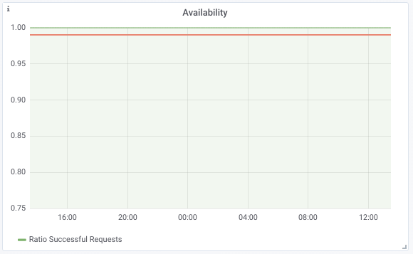
Given our SLO, we know we want to visualize the ratio of successful requests for availability and the 99th percentile of request times for latency. Fortunately, Grafana allows us to utilize PromQL, the Prometheus query language, to specify the expressions we want to graph.

For availability, we specify the following PromQL expression to graph the ratio of successful requests over the past hour:

sum(rate(caddy_http_response_status_count_total{service="blog",status!~"5.."}[1h])) /
sum(rate(caddy_http_response_status_count_total{service="blog"}[1h])) /

Over the last 24 hours, our graph displays the image below. As you can see, we did not fail a single request.

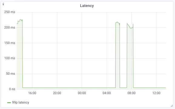
For latency, we specify the following PromQL expression to graph the 99th percentile of request time over the past hour:

histogram_quantile(0.99, sum(rate(caddy_http_request_duration_seconds_bucket[1h])) by (le))

Over the last 24 hours, our graph displays the image below. The 99th percentile request time maxes out just below 250ms, well below our SLO.

When we are exploring different visualizations, we want to interact directly with the Grafana UI. However, in the longer term, we want to place our dashboard's configuration under source control. Fortunately, Grafana allows us to export a dashboard's configuration as JSON, and then to specify a directory from which Grafana should load dashboard configuration on boot.

To utilize this strategy, we create another ConfigMap which we mount into our Grafana pod. As the ConfigMap is long, and almost entirely Grafana boilerplate, I won't embed it, but you can find it here if you're interested.

Conclusion

We're so close to being done implementing our SLO!

via GIPHY

The next blog post will cover our final step, which is configuring alerting around the percentage of error budget our application has burned. We'll also add a graph of error budget to our Grafana dashboard. After completing this step, we'll be extracting all the value we can from our instrumentation efforts. Can't wait to wrap this project up with y'all :)